Numerical differential equations (Euler, Runge-Kutta)

When a differential equation cannot be solved analytically, an approximate solution can be found using numerical methods. These methods compute the function values step by step from the differential equation and an initial condition. Two of the most common ones are Euler’s method and the Runge–Kutta method.

 

 

The idea behind numerical differential equations

A simple ordinary differential equation has the form:

 

$$ \large y' = f(x,y) $$

 

If an initial value \( \large y(x_0) = y_0 \) is known, \( \large f(x,y) \) can be used to calculate how \( y \) changes as \( x \) increases slightly. This process is repeated step by step, gradually building a numerical solution.

 

 

Euler’s method

Euler’s method is the simplest numerical solution. It uses the differential equation directly to calculate the next value as:

 

$$ \large y_{n+1} = y_n + h \cdot f(x_n, y_n) $$

 

Here \( \large h \) is the step size. By repeating the process with many small steps, an approximate curve of \( y(x) \) can be drawn.

 

 

Example of Euler’s method

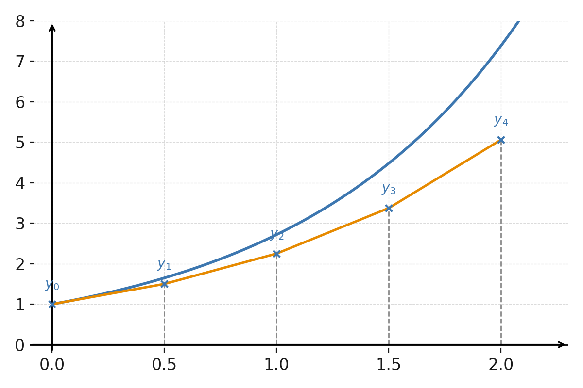
We want to solve \( \large y' = y \) with the initial condition \( \large y(0) = 1 \) and \( \large h = 0{,}5 \).

 

For each step:

 

$$ \large y_{n+1} = y_n + 0{,}5 \cdot y_n = 1{,}5y_n $$

 

After four steps we obtain:

 

$$ \large y_1 = 1{,}5, \quad y_2 = 2{,}25, \quad y_3 = 3{,}375, \quad y_4 = 5{,}0625 $$

 

The exact solution is \( \large y = e^x \), and for \( \large x=2 \) we get \( \large e^2 \approx 7{,}389 \). Euler’s method underestimates the true curve because each step uses a straight line instead of the curved function.

 

 

 

 

Runge–Kutta method (4th order)

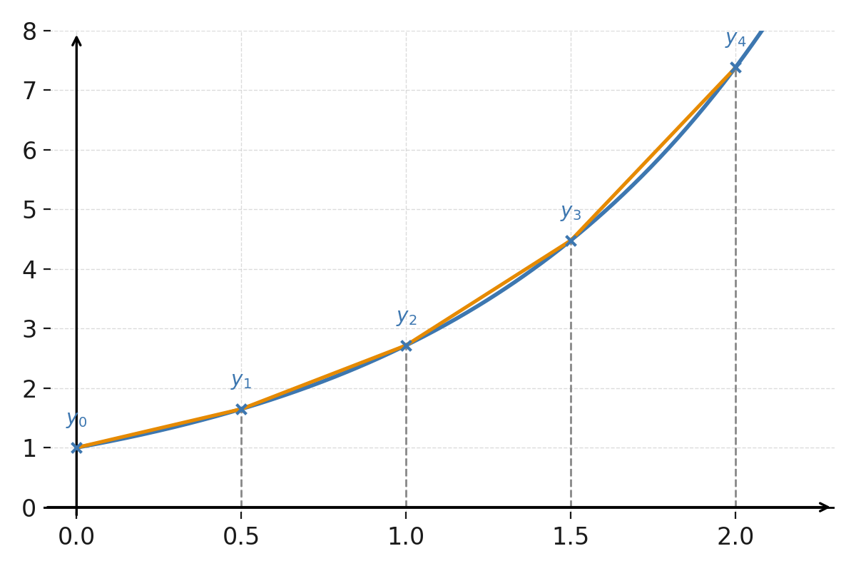
For better accuracy, the 4th order Runge–Kutta method (RK4) can be used. It takes the average of four slopes instead of just one:

 

$$
\large
\begin{aligned}
k_1 &= f(x_n, y_n) \\[8pt]
k_2 &= f\!\left(x_n + \frac{h}{2},\, y_n + \frac{h}{2}k_1\right) \\[8pt]
k_3 &= f\!\left(x_n + \frac{h}{2},\, y_n + \frac{h}{2}k_2\right) \\[8pt]
k_4 &= f\!\left(x_n + h,\, y_n + h k_3\right) \\[8pt]
y_{n+1} &= y_n + \frac{h}{6}\!\left(k_1 + 2k_2 + 2k_3 + k_4\right)
\end{aligned}
$$

 

RK4 is far more accurate than Euler’s method, even with few steps, and is therefore widely used in practice.

 

 

 

 

Remarks

Numerical differential equations are among the most important tools in applied mathematics, physics, and engineering. They are used to simulate systems where the rate of change is known but no closed-form expression for the function exists.