Linearization and approximation

Differential calculus makes it possible to understand and approximate functions locally. When a function is smooth and differentiable, it can be replaced by a straight line in a small region around a point – namely, the tangent line. This method is called linearization and is used to find quick approximations when exact calculations are difficult or unnecessary.

The idea behind linearization

Near a point $ \large x_0 $, a differentiable function $ \large f(x) $ behaves almost like its tangent. If one knows the function and its derivative at that point, the entire local behavior can be described by a linear function, which is easy to compute with.

The linear approximation (the tangent equation) has the form:

$$ \large f(x) \approx f(x_0) + f'(x_0) \cdot (x - x_0) $$

This expression says that the function value at a point close to $ \large x_0 $ can be approximated by the value at $ \large x_0 $ plus the change given by the slope $ \large f'(x_0) $. The closer $ \large x $ is to $ \large x_0 $, the better the approximation works.

Linearization tangent

Graphical understanding

The tangent line “touches” the graph of $ \large f(x) $ at one point and follows its direction there. For small changes in $ \large x $, the function and the tangent almost coincide. Linearization therefore means replacing a curved graph with its local straight line. This makes calculations much simpler without losing accuracy in that region.

Example 1: Linearization of a quadratic function

Find the linear approximation of $ \large f(x) = x^2 $ around the point $ \large x_0 = 2 $.

We have $ \large f(2) = 4 $ and $ \large f'(x) = 2x $, so $ \large f'(2) = 4 $. Thus:

$$ \large f(x) \approx 4 + 4(x - 2) = 4x - 4 $$

When $ \large x $ is close to 2, $ \large 4x - 4 $ is a good approximation of $ \large x^2 $. For example, $ \large f(2.1) \approx 4.4 $, while the exact value is $ \large 2.1^2 = 4.41 $.

Example 2: Approximation of a square root

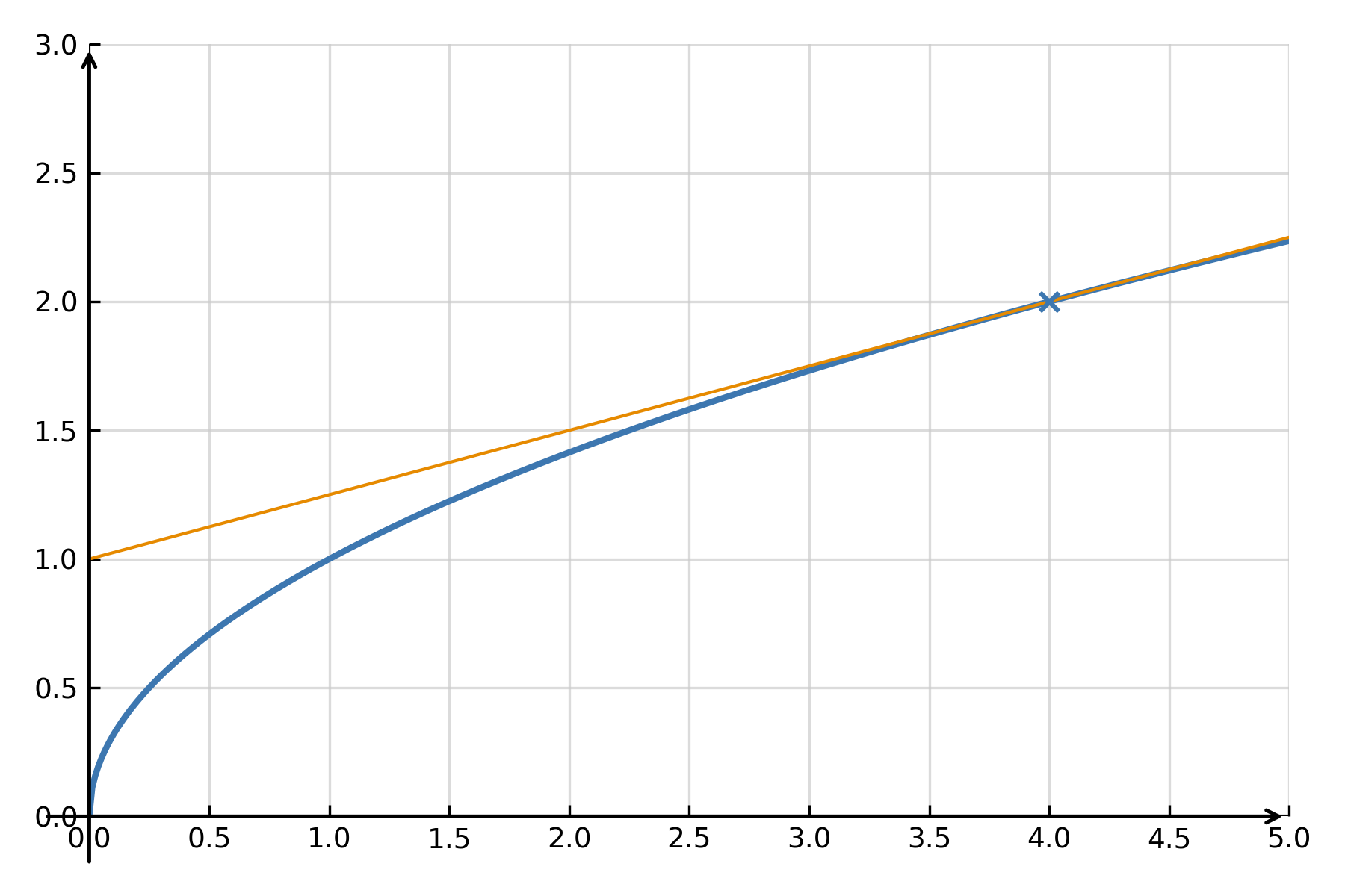
Linearization can be used to approximate square roots without a calculator. For example, $ \large \sqrt{4.1} $ can be found by linearizing the function $ \large f(x) = \sqrt{x} $ around $ \large x_0 = 4 $.

Here, $ \large f(4) = 2 $ and $ \large f'(x) = \frac{1}{2\sqrt{x}} $, so $ \large f'(4) = \frac{1}{4} $.

$$ \large f(x) \approx 2 + \frac{1}{4}(x - 4) $$

For $ \large x = 4.1 $: $ \large f(4.1) \approx 2 + \frac{1}{4} \cdot 0.1 = 2.025 $, while the exact value is $ \large 2.0248 $. The tangent approximation therefore gives a result with almost no error.

Error and accuracy

The closer $ \large x $ is to $ \large x_0 $, the better the approximation works. If one moves further away, the tangent line begins to deviate from the original curve because higher-order changes (curvature) become significant. This can be corrected by including more terms in a Taylor expansion.

To first order, linearization corresponds to the first part of the Taylor series:

$$ \large f(x) = f(x_0) + f'(x_0)(x - x_0) + \frac{f''(x_0)}{2!}(x - x_0)^2 + \dots $$

When only the first term after $ \large f(x_0) $ is taken, we get precisely the tangent approximation. Therefore, the method is also called the first-order Taylor approximation.

Example 3: Physical interpretation

In physics, linearization is used to describe motion or processes over short time intervals. If $ \large s(t) $ describes a position, the linear approximation

$$ \large s(t) \approx s(t_0) + v(t_0) \cdot (t - t_0) $$

can be interpreted as: “the new position is the old one plus velocity times time”. Here the velocity $ \large v(t_0) = s'(t_0) $ plays exactly the same role as the slope of the tangent in mathematics.

Summary

Linearization makes it possible to replace a function with a simple linear model around a given point. The tangent line acts as a local approximation that is quick to compute and often sufficiently accurate. The method forms the basis for many numerical procedures and for the Taylor expansion, which extends the idea to more precise approximations.