Differential equations

A differential equation describes the relationship between a function and its derivative. Instead of directly stating what the function is, it describes how the function changes. This makes differential equations a central tool in mathematics, physics, biology, and economics, where many phenomena involve changes over time.

 

 

What is a differential equation

An ordinary equation contains an unknown quantity, for example \( \large x \). A differential equation, on the other hand, contains an unknown function \( \large y(x) \) and its derivatives, such as \( \large y'(x) \) or \( \large y''(x) \). The goal is to find the function \( \large y(x) \) that satisfies the equation.

 

Examples:

 

$$ \large y' = 3x^2 $$

 

$$ \large y'' + y = 0 $$

 

The first equation states that the slope of \( \large y \) is always \( \large 3x^2 \). The second describes an oscillation, since it links the function with its own second derivative.

 

 

The basic idea

A differential equation does not directly tell how the graph of \( \large y \) looks, but how its slope changes from point to point. You can think of it as a recipe for motion or growth.

 

If the derivative is known, the function can be found by doing the opposite of differentiation – that is, by integrating. Therefore, differential equations are closely connected to integral calculus.

 

 

Orders and types

An ordinary differential equation (abbreviated ODE) involves only one independent variable, typically \( \large x \) or \( \large t \). If the equation includes several variables and derivatives with respect to several variables, it is called a partial differential equation (PDE).

 

The order of a differential equation is the highest derivative that appears. For example:

 

• \( \large y' = 3x^2 \) → first-order equation
• \( \large y'' + y = 0 \) → second-order equation

 

 

Solving simple differential equations

The simplest differential equations can be solved directly by integration. For example, if

 

$$ \large y' = 3x^2 $$

 

then \( \large y(x) \) can be found by integrating the right-hand side:

 

$$ \large y = \int 3x^2 \, dx = x^3 + C $$

 

Here \( \large C \) is the integration constant, representing all possible solutions — that is, all graphs with the same slope pattern but different vertical positions.

 

 

Separation of variables

A common method for solving first-order equations is separation of variables. If the equation can be written as

 

$$ \large \frac{dy}{dx} = g(x) \cdot h(y) $$

 

then \( \large x \) and \( \large y \) can be separated and integrated on each side:

 

$$ \large \int \frac{1}{h(y)} \, dy = \int g(x) \, dx $$

 

Example: Solve \( \large y' = 2xy \).

 

Separate the variables: \( \large \frac{1}{y} dy = 2x dx \).

 

Integrate both sides:

 

$$ \large \ln|y| = x^2 + C $$

 

Rewrite the general solution:

 

$$ \large y = A e^{x^2} $$

 

where \( \large A = e^C \) is a constant. This method works whenever the variables can be separated in this way.

 

 

Linear first-order differential equations

A linear first-order equation has the form:

 

$$ \large y' + p(x)y = q(x) $$

 

The solution is found by multiplying the entire equation by an integrating factor:

 

$$ \large \mu(x) = e^{\int p(x)\,dx} $$

 

This allows the equation to be written as

 

$$ \large (\mu(x)y)' = \mu(x)q(x) $$

 

and then integrated directly. This approach is called the integrating factor method.

 

 

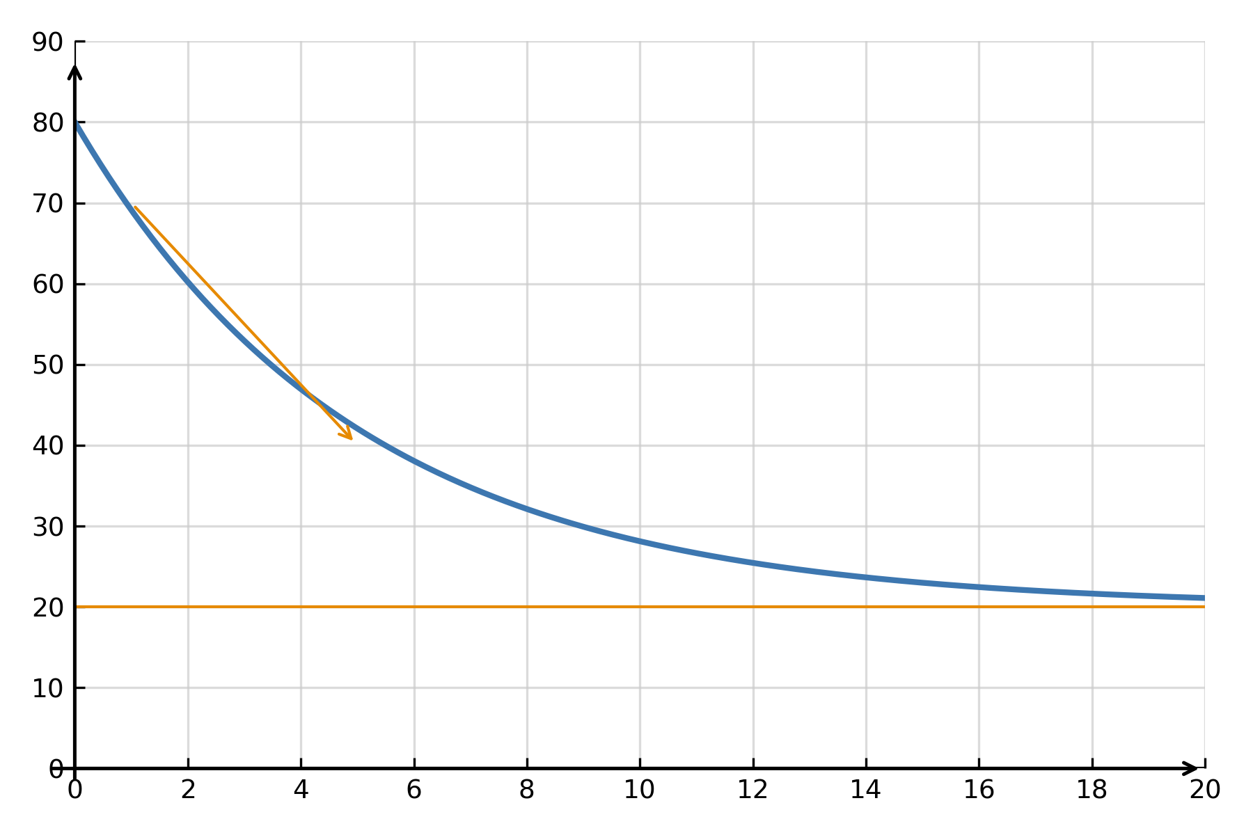
Example: Newton’s law of cooling

A classical example of a linear differential equation is Newton’s law of cooling:

 

$$ \large \frac{dT}{dt} = -k(T - T_{\text{env}}) $$

 

Here \( \large T(t) \) represents the temperature of an object that cools towards the surrounding temperature \( \large T_{\text{env}} \), and \( \large k \) is a constant. The solution shows that the temperature approaches the surroundings exponentially:

 

$$ \large T(t) = T_{\text{env}} + (T_0 - T_{\text{env}})e^{-kt} $$

 

Such an equation also appears in radioactive decay, capacitor discharge, and economic adjustment models.

 

 

 

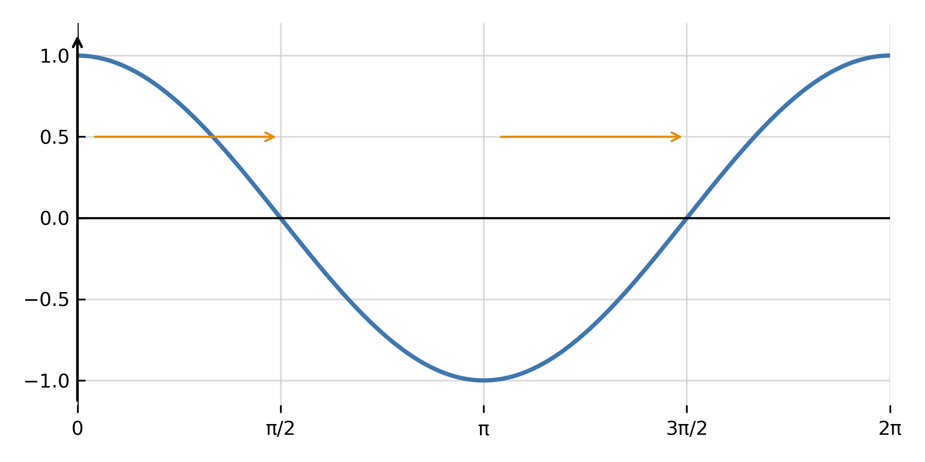
Second-order differential equations

When the second derivative is involved, the equation often describes motion or oscillations. An important example is harmonic oscillation:

 

$$ \large y'' + \omega^2 y = 0 $$

 

The solution is a combination of sine and cosine:

 

$$ \large y = A \cos(\omega x) + B \sin(\omega x) $$

 

Here \( \large A \) and \( \large B \) represent the initial conditions, while \( \large \omega \) gives the frequency of oscillation. This type of equation is used in mechanics, wave motion, and electrical circuits.

 

 

 

Numerical solutions

In many cases, a differential equation cannot be solved analytically. Instead, numerical methods are used, where the function is computed point by point from its derivative. The most well-known methods are Euler’s method, Runge–Kutta, and the Secant method, all explained in the section Numerical methods.

 

 

Summary

Differential equations describe how functions change and play a central role in applied mathematics. They are used to model growth, motion, oscillations, heat, current, and many other phenomena. Some can be solved by hand, while others require numerical methods, but all of them connect differential and integral calculus into one unified system.